Introduction to Basic Echo Doppler and Normal Cardiac Anatomy
Introduction to Echocardiography
Important Milestones in the Development of Echocardiography
- Lazzaro Spallanzani (1794)
- Studied bats’ use of ultrasound for navigation
- Jean Daniel Colladon (1826)
- Physicist used underwater church bell to calculate speed of sound
- Christian Doppler (1845)
- Theory of Doppler effect
- Pierre and Jacques Curie (1880)
- Discovered Piezo-Electric Effect
- Paul Langevin (1915)
- Physicist invented hydrophone to detect icebergs
- Karl Dussik (1942)
- Neurologist and first physician to use ultrasound (brain tumors)
The Development of Echocardiography
- A and B mode echocardiography (Hertz and Edler, 1953)
- M-mode echocardiography (early 1970s)
- 2-dimensional echocardiography (late 1970s)
- Doppler echocardiography (1980s)
- Pulse, continuous and color Doppler
2-Dimensional (2D) Echocardiography: non invasive assessment of intracardiac anatomy
- Available for fetal, neonatal, pediatric and adult patients
- Used to assess intracardiac anatomy for the presence of pathology
- Quantification of valve, chamber and vessel sizes
- Quantitative assessment of left ventricular function
- Systolic Function
- M-mode (fractional shortening)
- 2D volumetric assessment
- Simpson's biplane
- Bullet method
- Diastolic function
- Tissue Doppler
- Mitral E/A and E/E' ratios
- Pulmonary vein Ar to mitral A wave ratios
- Systolic Function
Ultrasound Basics
What is Ultrasound?
- A mechanical, longitudinal wave produced by passing electric current through a piezoelectric crystal
- Requires a medium for transmission
- Frequency exceeds the upper limit of human hearing (human hearing: 20-20,000 Hz)
- Diagnostic ultrasound frequency range: 2.5–14 MHz
- Ultrasound is free from radiation making it safe to use in fetuses, infants and children
Definition/Terminology
- Frequency: The number of cycles that occur during a particular duration of time. In ultrasound, described as cycles per second (also known at Hertz)
- Wavelength: The distance traveled by sound in one cycle or distance between two identical points in a wave cycle
- Period: The time required to complete a single cycle
- Amplitude: The magnitude of the pressure changes, i.e. the difference between the pressure peaks and nadirs (strength of the wave)
- Compression: area of high density
- Rarefication: area of low density
- $velocity = \lambda \times ƒ$
- v= velocity (constant for a given medium)
- ƒ= frequency (measured in hertz also known as Hz)
- λ = wavelengh
Frequency
Frequency refers to the number of cycles of compressions and rarefactions in a sound wave per second, with one cycle per second being 1 hertz.
Wavelength
- Distance traveled by sound in one cycle, or the distance between two identical points in the wave cycle.
- Inversely proportional to the frequency.
- Smaller wavelength = higher frequency = higher resolution = decreased penetration.
- This can be an important factor when choosing an echo probe to image a particular patient
Higher frequency probes (10–12 MHz)
- Poor penetration
- High resolution of structures closer to the probe
- Ideal for superficial structures or small infants
Lower frequency probes (2-7 MHz)
- Better penetration
- Lower resolution
- Ideal for deeper structures and better for older children
Sound Propagation
Sound waves are comprised of
- Compression (high air pressure)
- Compression refers to an area of high density
- Rarefaction (low air pressure)
- Rarefaction refers to area of low density
- Propagation velocity of sound is constant for a given medium and is dependent on the compressibility and density of the medium
- $V_s = \lambda \times ƒ$
| Material | Velocity of Sound $(m/s)$ |
|---|---|
| Air | 330 |
| Fat | 1450 |
| Water | 1480 |
| Human Soft Tissue (chest wall/heart) | 1540 |
| Brain | 1540 |
| Liver | 1550 |
| Kidney | 1560 |
| Blood | 1570 |
| Muscle | 1580 |
| Lens of eye | 1620 |
| Skull Bone | 4080 |
Ultrasound Production
Local tissue compression/decompression
- Propagates away from piezoelectric crystal in ultrasound probe at 1540 m/s in soft tissue
- Rate of compression/decompression determines frequency, typically 2.5–10 MHz
Piezoelectric Crystals
- Produce sound waves when electrically stimulated
- Produce electrical signals when sound waves received
- These electrical signals are converted into images
Ultrasound Propagation

- Absorption: Absorption is the most common form of attenuation. Absorption occurs as sound travels through soft tissue, the particles that transmit the waves vibrate and cause friction with subsequent loss of sound energy in the form of heat. In soft tissue, sound intensity decreases exponentially with depth.
- Refraction: Refraction describes reflection in which the sound wave hits the boundary of two tissues at an oblique angle. The reflections generated do not return directly back to the transducer. The angle of refraction is dependent on two things; the angle that the sound wave strikes the boundary between the two tissues and the difference in their propagation velocities. If the propagation velocity is greater in the first medium, refraction occurs towards the center, or perpendicular. If the velocity is greater in the second medium, refraction occurs away from the originating beam. In this instance, sound is not reflected directly back to the transducer and the image being depicted may not be clear, or potentially altered.
- Reflection: Reflection is categorized as specular or diffuse. Specular reflections represent large, smooth surfaces (i.e.- bone) where the sound wave is reflected back in a single direction. The greater the acoustic impedance between the two tissue surfaces, the greater the reflection and hence the brighter the echo will appear on ultrasound. Conversely, soft tissue is a diffuse reflector because adjoining cells create an uneven surface causing reflections to return in various directions in relation to the transmitted beam. However, because of the numerous surfaces, sound is able to get back to the transducer in a relatively uniform manner.
Dependent on:
- Incident angle: 90 degrees maximizes reflection
- Optimal for imaging of 2D structures
- Conversely, Doppler requires interrogation of structures parallel (between 0-20 degrees) to flow (see Doppler section below)
- Density: Dense materials reflect more
- Frequency: Higher frequency leads to higher absorption
Physics of Doppler
Doppler Effect
First described by Austrian physicist Christian Doppler in 1842
- When acoustic source moves relative to observer, frequencies of transmitted and observed waves are different
- Effective tool to measure tissue velocities
Why is it relevant?
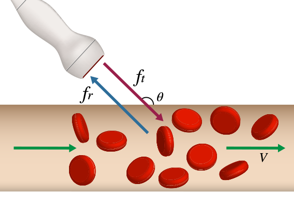
- Ultrasound is transmitted into a vessel and the sound that is reflected from the blood is detected.
- Blood is moving, therefore the sound undergoes a frequency (Doppler) shift.
Principles of Doppler
Beam of ultrasound hitting a moving object will be reflected back with a:
- Longer wavelength if the object is moving away
- Shorter wavelength if the object is moving towards
The faster the object of interest is moving the larger the Doppler shift.

Image reference: https://theglobalsoundproject.tumblr.com
Doppler Equation
$F_p = \frac{-2v \cos\theta F_t} {c}$
- $Fp =$ Frequency shift
- $Ft =$ transmit frequency
- $θ =$ angle between direction wave propagation and tissue motion
- $c =$ velocity of sound in soft tissue (1530 m/s)
Doppler Shift with Sound Waves
Affected by:
- Movement of ultrasound transmitter
- Movement of reflector
- Movement/properties of medium
Angle of incidence:
- If not at 0 degrees, error in measurement
- Acceptable limits of error are theta < 20 degrees (<6% error)
- If interrogating a vascular structure by Doppler, ideal to be as parallel to flow as possible (between 0-20 degrees) to avoid error in measurement
Principles of Doppler
$\Delta f = f_t - f_r = \frac{2 \times f_t \times V \times cos \theta} {C}$
Shift maxed for flows parallel to Doppler beam
- $V =$ velocity of flow
- $f_t =$ transmit frequency
- $f_r =$ return frequency
- $C =$ light constant
- $θ =$ angle between U/S beam and blood column
- At 0°: $cos \theta = 1$
- At 90°: $cos \theta = 0$
Ideal angle of interrogation should be close to 0°, but acceptable if less than 20 degrees
Effect of Doppler Angle
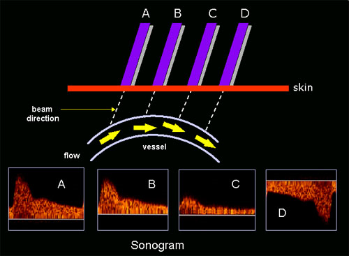
Effect of the Doppler angle in the sonogram. (A) higher-frequency Doppler signal is obtained if the beam is aligned more to the direction of flow. In the diagram, beam (A) is more aligned than (B) and produces higher-frequency Doppler signals. The beam/flow angle at (C) is almost 90° and there is a very poor Doppler signal. The flow at (D) is away from the beam and there is a negative signal.
Types of Doppler
Types of Doppler Ultrasound
- Pulse Wave
- Allows for sampling of velocity at a specific location of interest, but limited at higher velocities
High pulse repetition frequency (PRF)
- Allows for sampling of velocity at a specific location of interest, but limited at higher velocities
- Continuous Wave
- Allows sampling of highest peak velocity along the line of interrogation
- Lose ability to define exact location of specific velocities as sampling all velocities along line of interrogation
- Color Doppler
- Measures blood flow velocities
- Assesses flow into or within vessels or chambers
- Identifies regions of turbulent flow which may reflect stenosis
- Tissue Doppler
- Measures myocardial tissue velocities
- Surrogate for the assessment of diastolic function and can be blunted in the setting of diastolic dysfunction
Clinical Use of Doppler Echocardiography
Pulse and Continuous Wave Doppler
- Calculates mean and peak intracardiac gradients
- Valvar (e.g., pulmonary stenosis, aortic stenosis, mitral stenosis)
- Defects (ASD, VSD, PDA)
- Estimate RV and pulmonary artery pressures
Color Doppler
- Measures blood flow velocities
- Demonstrates normal laminar flow in unobstructed vessels and valves
- Demonstrates flow turbulence in narrowed vessels or across stenotic valves
- Can be used to quantify and assess mechanism of valve regurgitation
Tissue Doppler
- Detects myocardial tissue velocities
- Most commonly used for left ventricular lateral wall, interventricular septum and right ventricular free wall
- Decreased in diastolic dysfunction
Pulse and Continuous Wave Doppler
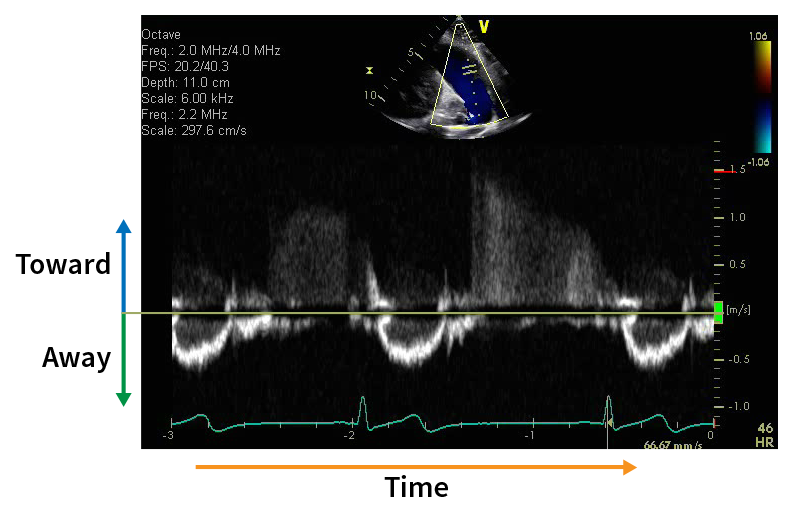
For PW and CW Doppler:
- X axis is Time
- Y axis is Velocity
- Moving toward is above the 0 line
- Moving away is below the 0 line
Tips for Optimizing Pulse Doppler
- Minimize angle of incidence
- Use low frequency transducer
- Shift baseline away from direction of flow
- Use shallowest depth setting
- Narrow interrogation sector to maximize frame rate
- Set to high PRF
Pulse Repetition Frequency (PRF)
- The PRF is the number of pulses (send and listen cycles) of ultrasound sent out by the transducer per second.
- Also known as sampling frequency
- It is dependent on:
- Velocity of sound
- Depth of tissue being interrogated
The deeper the tissue being examined, the longer the transducer has to wait for echoes to come back, hence a lower PRF.
- High PRF
- Probe emits 2nd signal prior to receiving first
- If still get aliasing consider CW Doppler
Nyquist Limit
- Highest detectable velocity
- It is equal to ½ PRF (pulse repetition frequency)
- Exceeding this limit creates aliasing
- Doppler signal appears to "wrap around"
- Unable to accurately quantify true maximum velocity in this setting
Exceeding the Nyquist Limit: Aliasing
Aliasing
- The inability to detect large Doppler shift is known as aliasing.
- If velocity of scattering object is large and shift between subsequent acquisitions > ½ wavelength
- PW Doppler ineffective at differentiating velocities
- Methods to limit aliasing
- Shallower depth
- Continuous wave Doppler
- Lower frequency transducer
- Increase scale
- Move baseline up or down
- Down (if Doppler signal of interest is above baseline)
- Up (if Doppler signal of interest is below baseline)
- Increase PRF
- Compromise must be made between velocity resolution and maximal detectable velocity
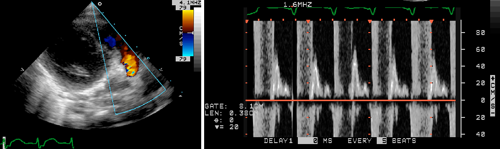
Pulse Wave Doppler
- US signals sent at regular intervals (PRF) along ultrasound line
- Based on frequency of reflected signals off RBCs, velocity signal is obtained
- Range resolution
- Move sample volume and localize velocity to specific region
- Velocity determined only at point of interest or “sample gate”
- Limited velocities PW can accurately measure
- Higher velocities cause aliasing (if Doppler shift exceeds ½ PRF)
- Two horizontal lines represent the sample gate
- Doppler waveform has hollowed out appearance
- Low velocity
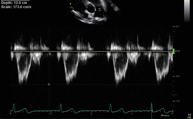
Continuous Wave Doppler
- One piezoelectric crystal transmits continuous wave of mixed frequency
- Second crystal records continuously reflected signals
- Sampling rate is infinite
- Can measure high velocity signals
- Useful for measuring peak velocities
- Unable to localize velocity along beam signal
- All velocities within scan line contribute to reflected signal and displayed on spectrogram leading to range ambiguity
- Beware of measuring wrong signal
- Velocities close to transducer contribute more than those further away
- No range gating (denoted by single circle or single horizontal line in spectral Doppler)
- All velocities along scan line sampled
- Doppler signal is well filled in
- High velocity
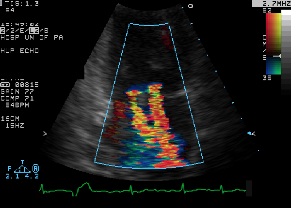
Color Doppler
- Uses multiple pulse wave signals to assess multiple sample volumes
- Codes mean velocities at each sample gate
- Real time image of blood flow
- Color flow measures local spectrum of velocities
- Blood flow is color coded
- Red: towards transducer
- Blue: away from transducer
- Filter is applied to remove slow moving structures (cardiac walls)
- Good for rapidly providing a gestalt of laminar versus disturbed flows and direction of flow in a real time image
- It is important to adjust the nyquist limit depending on structure being interrogated
- Setting a nyquist limit too low is larger vasculature with higher velocities (i.e.- aorta) may result in the false appearance of turbulent/disturbed flow patterns
- Need to decrease nyquist limit to assess flow within smaller vessels with lower velocities (i.e.- pulmonary veins and coronary arteries)
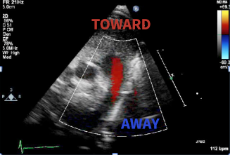
Red moving toward the transducer
- Allows sampling of larger area
- Width and depth of color jet
- Direction of color jet
- Detect multiple jets
- Limited temporal resolution
- Narrow width of interrogation to improve frame rate
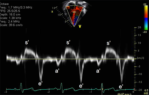
Tissue Doppler Imaging
- Can be performed in pulse wave and color modes.
- Measures peak myocardial velocities
- Angle dependent measurement
- Used in apical four chamber view to access long-axis ventricular motion
- Longitudinally oriented endocardial fibers are most parallel to the ultrasound beam in the apical views.
- Mitral annular motion is a good surrogate measure of overall longitudinal left ventricular (LV) contraction and relaxation.
- Provides assessment of diastolic function
- Less load dependent than standard Doppler techniques.
- Sa: Systolic myocardial motion
- Ea: Velocity of early myocardial relaxation as the mitral annulus ascends during early rapid LV filling.
- Aa: Atrial contraction
Bernoulli Equation

$P_1 - P_2 = 4(V_2^2 - V_1^2)$
As fluid passes through an obstruction total drop in pressure due to:
- Convective acceleration
- Conversion to kinetic energy
- Energy loss
- Friction of fluid against wall (viscous losses)
- From acceleration of fluid
Fluid acceleration, viscosity, and $V_1$ ignored in simplified equation
EXCEPTION: V1 cannot be ignored in the setting of multiple areas of obstruction in series
Modified Bernoulli Equation
$\text{Pressure gradient} = 4V^2$
$V = \text{peak velocity}$
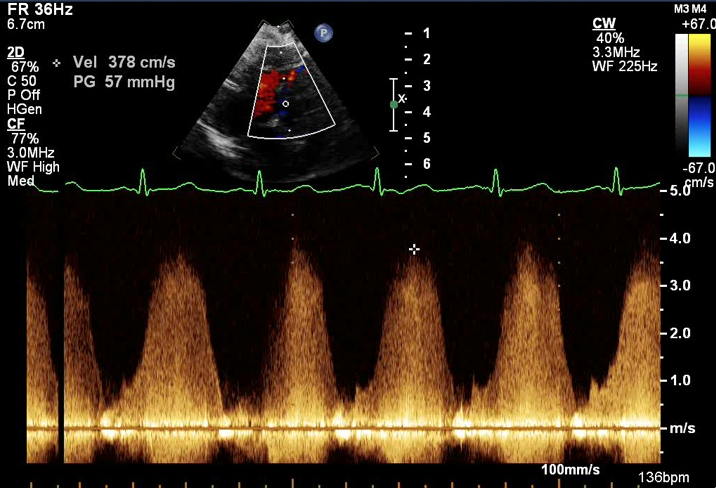
Spectral Doppler of Tricuspid Regurgitation (TR)
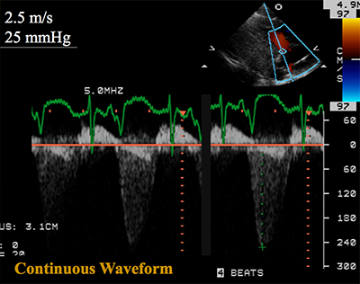
Estimate of RVP/PA Pressures
$\operatorname{Pressure gradient} = \operatorname{RVP} – \operatorname{RAP}$
$\operatorname{RVP} = \operatorname{RAP} + \textrm{ pressure gradient}$
$\operatorname{RVP} = 5 \textrm{ mmHg} \small\text{ (assumed normal RA pressure)}\normalsize + 25 \textrm{ mmHg}$
$\operatorname{RVP} = 30 \textrm{ mmHg}$
- TR jet can also be used to estimate the systolic pulmonary arterial pressure in an anatomically normal heart without right sided obstructive lesions
- Pulmonary regurgitation spectral Doppler tracing can be used to estimate PA end diastolic and mean PA pressures
Modified Bernoulli Equation Applications
$\operatorname{RVSP} = 4(\operatorname{TR})^2 + \operatorname{RAp}$
$\operatorname{RVSP} = \operatorname{SBP} – 4(\operatorname{VSD})^2$
$\operatorname{PA EDP} = 4(\operatorname{PR})^2 + \operatorname{RAp}$
$\operatorname{LVSP} = 4(\operatorname{MR})^2 + \operatorname{LAp}$
| $\text{RVSP}$ | Right ventricular systolic pressure |
|---|---|
| $\text{LVSP}$ | Left ventricular systolic pressure |
| $\text{PA EDP}$ | Pulmonary artery end diastolic pressure |
| $\text{SBP}$ | Systolic blood pressure |
| $\text{TR}$ | Tricuspid regurgitation peak velocity |
| $\text{MR}$ | Mitral regurgitation peak velocity |
| $\text{PR}$ | Pulmonary regurgitation peak end diastolic velocity |
| $\text{VSD}$ | Peak spectral Doppler velocity across VSD |
| $\text{RAp}$ | Right atrial pressure |
| $\text{LAp}$ | Left atrial pressure |
Cardiac Morphology: The Cardiac Chambers
Cardiac chambers are identified in terms of their internal morphology and not in terms of other cardiac structures or by their spatial relationships
Important to use the most constant component to distinguish the identity of a chamber and not to use variable features
Right Atrium
Anteriorly located
Broad based triangular atrial appendage
Septum secundum
Receives the IVC, SVC and coronary sinus
Extensive pectinate muscles extend outside appendage towards tricuspid valve
Left Atrium
Posteriorly located
Long and narrow finger-like posterior atrial appendage
Flap of fossa ovalis (septum primum)
Receives pulmonary veins (majority of time, however, this can vary in the setting of anomalous pulmonary venous drainage)
Pectinate muscles confined to the left atrial appendage
Right Ventricle
Thin walled
Tripartite configuration
Coarse trabeculations (particularly towards the apex)
Presence of a moderator band (band of muscle that runs from the septum to the lateral wall of the right ventricle)
Trileaflet atrioventricular valve (tricuspid valve)
Lower more apically positioned septal leaflet attachment of tricuspid valve
Tricuspid valve chordae insert to the interventricular septum and indistinct papillary muscles (septophilic)
Fibrous discontinuity between tricuspid and pulmonary valve (subpulmonary conus)
Left Ventricle
Smooth walled
Bullet shaped configuration
Fine trabeculations
No moderater band
Bileaflet atrioventricular valve (mitral valve)
Higher, more basally positioned mitral valve
Fibrous continuity with mitral and aortic valve (absent conus)
The mitral valve attaches to two distinct papillary muscles which insert to the LV free wall
Absence of mitral valve attachments to the interventricular septum (septophobic)